What Must The Rate Of Money Growth Equal In Order To Achieve This Zero-inflation Goal?

11.1 The Quantity Theory of Money

Learning Objectives

After you lot have read this section, you should be able to answer the following questions.

1. What is the quantity theory of money?
2. What is the classical dichotomy?
3. According to the quantity theory, what determines the inflation rate in the long run?

Nosotros begin by presenting a framework to highlight the link between money growth and inflation over long periods of fourth dimension.The framework complements our discussion of inflation in the brusque run, contained in Chapter 10 "Agreement the Fed". The quantity theory of moneyA relationship among coin, output, and prices that is used to written report aggrandizement. is a human relationship among money, output, and prices that is used to written report inflation. It is based on an accounting identity that can be traced dorsum to the round flow of income. Among other things, the circular period tells us that

nominal spending = nominal gross domestic product (GDP).

The "nominal spending" in this expression is carried out using money. While money consists of many unlike assets, you can—every bit a metaphor—recollect of coin as consisting entirely of dollar bills. Nominal spending in the economy would then take the class of these dollar bills going from person to person. If there are not very many dollar bills relative to total nominal spending, then each bill must exist involved in a big number of transactions.

The velocity of moneyNominal GDP divided by the money supply. is a measure of how rapidly (on boilerplate) these dollar bills modify hands in the economy. It is calculated by dividing nominal spending by the coin supply, which is the full stock of money in the economy:

$$\text{velocity of money}=\frac{\text{nominal spending}}{\text{money supply}}=\frac{\text{nominal GDP}}{\text{money supply}}\text{.}$$

If the velocity is high, and so for each dollar, the economy produces a large amount of nominal Gross domestic product.

Using the fact that nominal GDP equals real GDP × the toll level, nosotros see that

$$\text{velocity of money}=\frac{\text{price level × real Gross domestic product}}{\text{money supply}}\text{.}$$

And if we multiply both sides of this equation past the money supply, we get the quantity equationAn equation stating that the supply of money times the velocity of money equals nominal Gdp. , which is one of the most famous expressions in economics:

money supply × velocity of money = cost level × real Gross domestic product.

Let us see how these equations work past looking at 2005. In that year, nominal Gross domestic product was most $13 trillion in the United States. The amount of coin circulating in the economy was near $vi.5 trillion.In Chapter 9 "Coin: A User's Guide", nosotros discussed the fact that in that location is no simple single definition of money. This figure refers to a number called "M2," which includes currency and likewise deposits in banks that are readily accessible for spending. If this money took the form of 6.5 trillion dollar bills changing hands for each transaction that we count in Gdp, and then, on average, each bill must have inverse hands twice during the year (13/6.5 = 2). So the velocity of money was 2 in 2005.

The Classical Dichotomy

And then far, we take only written a definition. There are two steps that take u.s. from this definition to a theory of inflation. Beginning we use the quantity equation to requite us a theory of the price level. And so we examine the growth rate of the price level, which is the inflation charge per unit.

In macroeconomics we are e'er careful to distinguish betwixt nominal and real variables:

• Nominal variablesA variable divers and measured in terms of money. are defined and measured in terms of money. Examples include nominal GDP, the nominal wage, the dollar toll of a carton of milk, the toll level, and so forth. (Nearly nominal variables are measured in monetary units, but some are just numbers. For example, the nominal interest rate tells you how many dollars yous volition obtain side by side yr for each dollar you invest in an asset this year. Information technology is thus measured as "dollars per dollar," and so it is a number.)
• All variables not defined or measured in terms of money are real variablesA variable defined and measured in terms other than money, often in terms of existent GDP. . They include all the variables that nosotros divide by a price index in order to right for the effects of aggrandizement, such as real Gross domestic product, real consumption, the capital stock, the real wage, and so forth. For the sake of intuition, you can recall of these variables as being measured in terms of units of (base of operations year) GDP (then when we talk about existent consumption, for example, you tin can remember about the bodily consumption of a bundle of goods and services past a household). Real variables also include the supply of labor (measured in hours) and many variables that have no specific units but are simply numbers, such as the velocity of money or the capital letter-to-output ratio of an economy.

Prior to the Great Depression, the dominant view in economic science was an economic theory called the classical dichotomyThe dichotomy that existent variables are determined independently of nominal variables. . Although this term sounds imposing, the idea is not. According to the classical dichotomy, real variables are determined independently of nominal variables. In other words, if you take the long list of variables used by macroeconomists and write them in ii columns—existent variables on the left and nominal variables on the right—then you tin effigy out all the existent variables without needing to know any of the nominal variables.

Following the Great Low, economists turned instead to the amass expenditure modelThe relationship between planned spending and output. to meliorate understand the fluctuations of the aggregate economy. In that framework, the classical dichotomy does not hold. Economists still believe the classical dichotomy is important, merely today economists call up that the classical dichotomy merely applies in the long run.

The classical dichotomy tin exist seen from the following thought experiment. Starting time with a state of affairs in which the economic system is in equilibrium, meaning that supply and demand are in balance in all the different markets in the economy. The classical dichotomy tells us that this equilibrium determines relative prices (the price of one skilful in terms of another), non absolute prices. We tin can understand this effect by thinking well-nigh the markets for labor, goods, and credit.

Figure xi.2 "Labor Market Equilibrium" presents the labor market place equilibrium. On the vertical axis is the real wage because households and firms brand their labor supply and need decisions based on existent, non nominal, wages. Households desire to know how much additional consumption they can get by working more, whereas firms desire to know the price of hiring more labor in terms of output. In both cases, it is the real wage that determines economic choices.

Effigy 11.2 Labor Market place Equilibrium

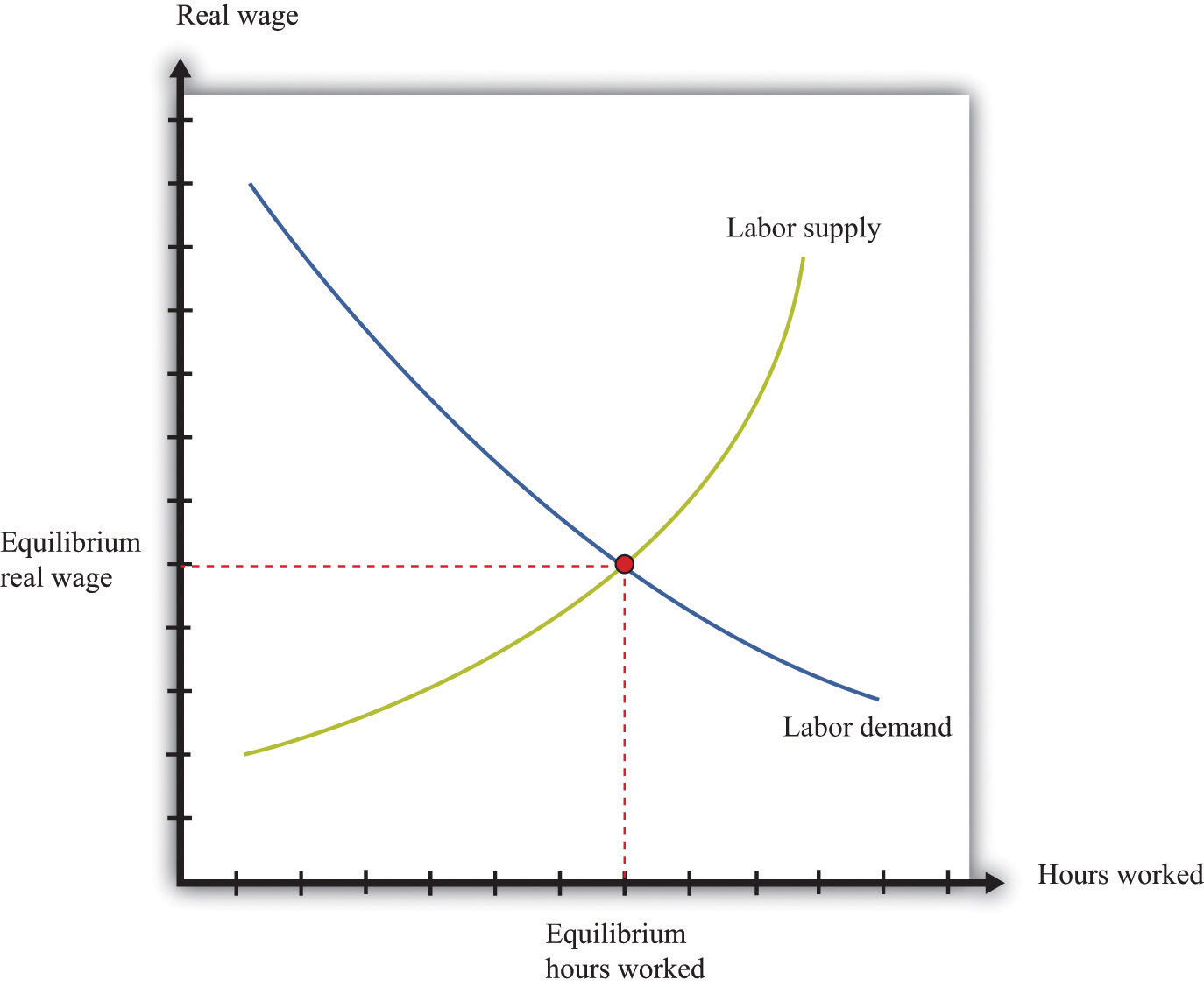
Now think about the markets for appurtenances and services. The need for any good or service depends on the real income of households and the real price of the skillful or service. We can calculate real prices past correcting for inflation: that is, past dividing each nominal price past the amass price level. Household demand decisions depend on real variables, such as real income and relative prices.If yous have studied the principles of microeconomics, call up that the budget constraint of a household depends on income divided by the cost of one good and on the price of one skilful in terms of another. If there are multiple appurtenances, the budget constraint can be determined past dividing income past the price level and by dividing all prices by the same price level. The same is truthful for the supply decisions of firms. We have already argued that labor demand depends on simply the existent wage. Hence the supply of output also depends on the real, not the nominal, wage. More than generally, if the house uses other inputs in the production process, what matters to the firm's conclusion is the price of these inputs relative to the cost of its output, or—more than generally—relative to the overall toll level.If yous take studied the principles of microeconomics, the status that toll equals marginal price is used to characterize the output decision of a business firm. What matters then is the price of the input, relative to the price of output.

What nearly credit markets? The supply and demand for credit depends on the real interest charge per unit. This means that those supplying credit think about the return they receive on making loans in real terms: although the loan may be stated in terms of coin, the supply of credit really depends on the existent render. The same is true for borrowers: a loan contract may stipulate a nominal interest rate, but the existent interest rate determines the cost of borrowing in terms of appurtenances. The supply of and demand for credit is illustrated in Figure 11.3 "Credit Market Equilibrium".

Figure xi.3 Credit Market place Equilibrium

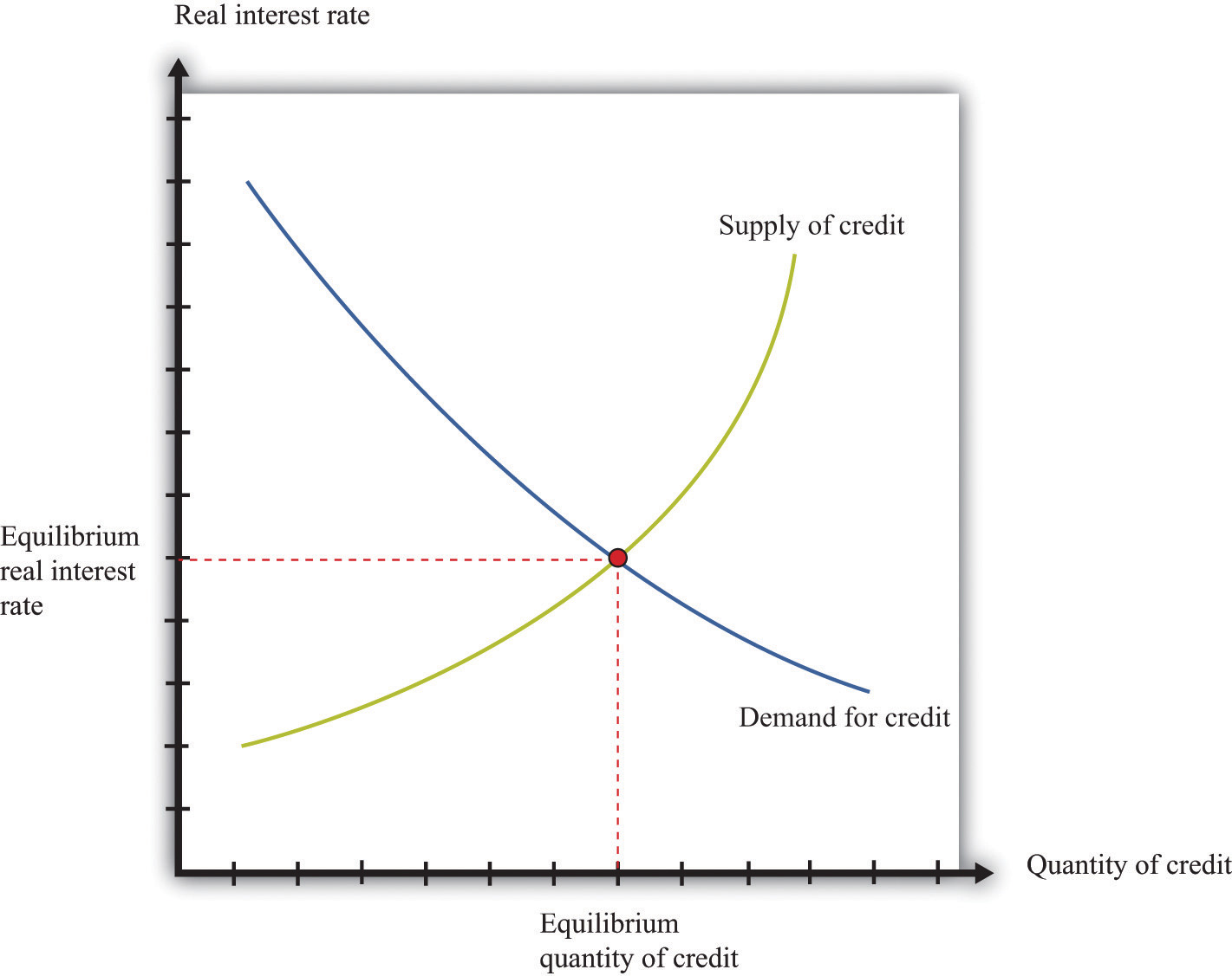
The credit market equilibrium occurs at a quantity of credit extended (loans) and a real interest charge per unit where the quantity supplied is equal to the quantity demanded.

The classical dichotomy has a primal implication that nosotros tin study through a comparative statics exercise. Recall that in a comparative statics practise we examine how the equilibrium prices and output change when something else, exterior of the market place, changes. Hither we ask: what happens to real Gross domestic product and the long-run price level when the money supply changes? To discover the reply, we brainstorm with the quantity equation:

coin supply × velocity of coin = price level × real Gross domestic product.

Previously we discussed this equation every bit an identity—something that must be true by the definition of the variables. Now we plough it into a theory. To do and then, we make the supposition that the velocity of money is fixed. This ways that any increase in the coin supply must increase the left-hand side of the quantity equation. When the left-manus side of the quantity equation increases, and then, for whatsoever given level of output, the price level is higher (equivalently, for any given value of the price level, the level of real GDP is higher).

What then changes when nosotros change the money supply: output, prices, or both? Based on the classical dichotomy, we know the respond. Existent variables, such equally real GDP and the velocity of money, stay constant. A alter in a nominal variable—the money supply—leads to changes in other nominal variables, merely existent variables exercise not change. The fact that changes in the money supply take no long-run issue on real variables is called the long-run neutrality of moneyThe fact that changes in the money supply have no long-run result on real variables. .

How does this view of the effects of monetary policy fit with the monetary transmission mechanismA mechanism explaining how the actions of a key depository financial institution impact amass economic variables, in particular real GDP. ?See Chapter 10 "Understanding the Fed". The monetary transmission machinery explains that the monetary authorization affects aggregate spending by changing its target interest rate.

• The monetary authority changes involvement rates.
• Changes in interest rates influence spending on durables by firms and households.
• Changes in spending influence aggregate spending through a multiplier outcome.

Retrieve that the monetary authorisation changes interest rates through open-market operations. If it wants to boost aggregate spending, information technology does and then past cutting interest rates, and it cuts interest rates by purchasing government bonds with money. An interest rate cut is equivalent to an increase in the supply of money, so the budgetary manual mechanism as well teaches united states of america that an increase in the supply of money leads to an increase in aggregate spending.There is one divergence, unimportant here, which is that the budgetary manual machinery does not necessarily suppose that the velocity of money is constant. The monetary manual machinery is useful when we want to sympathize the short-run furnishings of budgetary policy. When studying the long run, it is easier to work with the quantity equation and to think about monetary policy in terms of the supply of money rather than involvement rates.

Finally, a reminder: in the brusk run, the neutrality of money does not hold. This is considering in the brusk run we assume stickiness of nominal wages and/or prices. In this case, changes in the nominal coin supply will lead to changes in the existent money supply. With gummy wages and/or prices, the classical dichotomy is broken.

Long-Run Inflation

We now apply the quantity equation to provide the states with a theory of long-run aggrandizement. To practice then, we utilise the rules of growth rates. Ane of these rules is as follows: if you accept two variables, 10 and y, then the growth rate of the product (10 × y) is the sum of the growth charge per unit of x and the growth rate of y. We can employ this to the quantity equation:

money supply × velocity of coin = price level × existent GDP.

The left side of this equation is the product of two variables, the money supply and the velocity of money. The right side is likewise the product of two variables. So we obtain

growth charge per unit of the money supply + growth rate of the velocity of money = inflation rate + growth charge per unit of output.

Nosotros accept used the fact that the growth rate of the price level is, by definition, the aggrandizement rate.

Nosotros continue to assume that the velocity of money is a constant.In fact, the velocity of coin might also grow over time as a outcome of developments in the financial sector. Proverb that the velocity of money is abiding is the same as maxim that its growth rate is naught. Using this fact and rearranging the equation, we discover that the long-run aggrandizement charge per unit depends on the difference between how rapidly the money supply grows and how rapidly output grows:

inflation rate = growth rate of money supply − growth rate of output.

The long-run growth rate of output does not depend on the growth charge per unit of the coin supply or the inflation charge per unit. We know this considering long-run output growth depends on the aggregating of capital, labor, and engineering. From our discussion of labor and credit markets, equilibrium in these markets is described past real variables. Equilibrium in the labor market depends on the existent wage and not on any nominal variables. Likewise, equilibrium in the credit market tells us that the level of investment does not depend on nominal variables. Since the capital stock in any period is just the aggregating of past investment, we know that the stock of capital is also independent of nominal variables.

Therefore there is a direct link between the money supply growth rate and the inflation rate. The classical dichotomy teaches us that changes in the coin supply practice not bear on the velocity of money or the level of output. It follows that any changes in the growth charge per unit of the money supply will show up one-for-one as changes in the inflation rate. We say more near monetary policy later, just find that there are immediate implications for the conduct of monetary policy:

• In a growing economy, there are more transactions taking identify, so there is typically a need for more money to facilitate those transactions. Thus some growth of the coin supply is probably desirable to match the increased income.
• If the budgetary regime desire a stable price level—zero aggrandizement—in the long run, then they should try to set the growth rate of the money supply equal to the (long-run) growth rate of output.
• If the monetary regime want a low level of aggrandizement in the long run, then they should aim to take the money supply grow just a piffling flake faster than the growth rate of output.

Go along in listen that this is just a theory. The quantity equation holds as an identity. But the supposition of constant velocity and the statement that long-run output growth is contained of coin growth are assertions based on a body of theory. We at present await at how well this theory fits the facts.

Key Takeaways

1. The quantity theory of money states that the supply of money times the velocity of money equals nominal GDP.
2. According to the classical dichotomy, real variables, such as existent Gross domestic product, consumption, investment, the real wage, and the real involvement charge per unit, are determined independently of nominal variables, such as the coin supply.
3. Using the quantity equation along with the classical dichotomy, in the long run the inflation charge per unit equals the rate of money growth minus the growth rate of output.

Checking Your Understanding

1. Is the real wage a nominal variable? What about the coin supply?
2. If velocity of money decreases by two percent and the money supply does not grow, can y'all say what will happen to nominal GDP growth? Can you say what volition happen to inflation?

Source: https://saylordotorg.github.io/text_macroeconomics-theory-through-applications/s15-01-the-quantity-theory-of-money.html

Posted by: mcnamaraformoush.blogspot.com

Share this post